How can a machine learn? An introduction to artificial intelligence
- Andrew Daniel

- Aug 13, 2020
- 11 min read
Updated: Aug 14, 2020
Teaching a machine to learn
One of the most famous problems in artificial intelligence is to teach a computer so that it can recognise pictures of cats. For example, we would like a computer to recognise that this is a cat:

and this is not a cat:

This is called a classification problem: to identify whether something is true (the image is a cat) or false (the image is not a cat).
We need to input the images into our computer, then program our computer to make a set of calculations on the image, and then our computer should output either true or false.
We can create the inputs by looking at the data in the image. In a computer an image is just a set of pixels – coloured points. Each pixel can hold three numbers to tell the computer the amount of red, green and blue at the point: these are called RGB values. For example (1, 0, 0) would be pure-red (all red, no green, no blue), (0, 1, 0) would be pure-green, and (0.5, 0.5, 0.5) would be a shade of grey.
Let’s say we have an image which is 64 x 64 pixels in size (the typical size of a small image on the internet). At each pixel we have three numbers for the RGB values, so in total there are 64 x 64 x 3 = 12288 numbers which are needed to represent the image in our computer.
This list of 12288 numbers will be the inputs to our computer program.
Our computer then needs to make a set of calculations on the inputs, and we will call these calculations a Neural Network. In a later blog we will study the mathematics of a neural network in detail.
The neural network then needs to output a single number: 1 (if the computer thinks the image shows a cat) or 0 (if the computer thinks that the image doesn’t show a cat).
This diagram shows the idea of our computer program:

And that’s the basic idea of a cat recogniser in artificial intelligence. More accurately, we will use the term Machine Learning rather than artificial intelligence ……. because we are trying to teach a machine to learn!
However, we need first to understand the mathematical ideas involved in a neural network, so ……
Let’s start with a much simpler problem ……..
We’ll imagine a physics experiment with a container full of liquid. We can control the temperature of the liquid, and, as the temperature changes, we can measure how the pressure of the liquid changes.
In this case there is just one input, temperature, rather than the 12288 inputs we need to recognise cats, and one output, pressure. Pressure can now have range of values, while in our cat recogniser the only values for the output were 1 and 0.
We conduct a series of experiments, and the data that we get for temperature and pressure is shown below:

(For our purposes we don’t need to worry about the units of temperature and pressure).
We would like to use our graph to make predictions of the pressure for a particular temperature. For a human, with just one input, this is easy: we just draw a line of best fit on the graph, and then use it to make predictions:

For example, the red dashed line shows that if the temperature is 4.5, then we would predict a pressure of 4.5 also.
However, in machine learning we are trying to do something quite different: we are trying to teach a computer to learn how to make the predictions – without explicitly programming it to draw a line of best fit.
A good way to teach our computer is to ask it to do a very large number of trials with different random lines, and then to work out which lines are best at fitting the data. In other words, our computer will be learning about how to draw a line of best fit.
Machine learning to fit data
We can start by asking our computer to try equations for the line which are of the form

where P is the predicted pressure, T is the temperature, and w is a number that will correspond to the gradient of the straight line on the graph. The letter w is usually used in machine learning because, as you’ll see, it corresponds to the weight in part of a neural network.
In this first simple example we haven’t added another term onto the end of the equation, corresponding to a y-intercept, although we will add this later. For now, we are using line with a gradient that can vary, but the lines must all pass through the origin of the graph.
We will ask our computer to try lots of different equations, with random values of w. For example, if the computer decides to use w = 2 then our data with the line fitted onto it (the red line) looks like this:

If our computer chooses w = 0.5 then the graph looks like this:

Neither of these values of w give the computer a good fit to the data, but these graphs are still an important part of the process for our computer to learn.
If the computer decides to try w = 1.05, the fit looks much more accurate:

How good is the fit? The Cost Function
Now that our computer is trying lots of different lines to fit the data, for different values of w, we need to give our computer a way to measure how accurately a line has fitted the data. For now, we will do this with a simple calculation:
· For each data point, work out the difference between the predicted pressure and the actual pressure in the experience
· Square each of these differences
· Add up these squared differences to find the total: we will call this the cost function.
We can show this in an equation:

where y is the predicted pressure and P is the actual pressure. ∑ is a Greek letter, sigma, used in mathematics to show that we are adding up all of the squared differences.
We square the differences so that negative values of the difference don’t just act to cancel out positive values of the difference. This is the same method used to calculate variance and standard deviation, for example. However, it turns out that in machine learning using squared differences isn’t the best way to measure the accuracy of fit – a later blog will show a better way to do this using logarithms.
The cost function gives us a single number which represents how accurately a line has fitted the data. A large value for the cost function means that the line has fitted out data badly, like the graphs for w = 2 and w = 0.5 above. A small value for the cost function means that the computer has created a better fit, like the graph for w = 1.1.
If our computer now plots a graph of the cost for all of the many different values of w that it tried, the graph looks like this:

This graph shows that the cost is smallest for a value of w around 1, where there is a minimum turning point in the graph. We need to teach our computer to find this minimum turning point, so that it can then use the best value of w in order to make predictions.
If you’ve studied calculus and differentiation, you will know that in some situations you can find the position of a turning point by setting the derivative of the graph to 0, and solving the resulting equation.
However, in this case the computer doesn’t have an equation that it can differentiate – it just has a series of values of w and the corresponding values of cost that it has worked out. To find the minimum turning point we will need to teach our computer a different method.
Finding the minimum on a graph: gradient descent
Machine learning uses a technique called gradient descent to find the minimum point. With just one variable, the weight w which can be changed to lots of different values, this is an easy method to use. With a large number of variables, like in our cat recogniser problem, you’ll see that it’s a bit more more tricky to use.
We start at a random value of w, giving a point on the cost graph, and compute the gradient at that point. To compute the gradient we use a numerical method: take two points on the graph very close to each other, and calculate the gradient of the straight line between the points. This gives us the gradient of the tangent (shown in red below) to the curve at that point:

(If you would like to research numerical differentiation in more detail, you may find it useful to read about the Newton-Raphson method, https://en.wikipedia.org/wiki/Newton%27s_method.)
If this starting random value of w is called w0, we can calculate a second value of w, called w1, by taking a step down the tangent:

In this equation m0 is the gradient of the cost function at the starting point w0 and α is called the learning rate. The size of α determines how quickly we can move along the cost curve on the graph towards the minimum turning point.
Applying this equation moves a single step down the cost curve, towards the minimum turning point:

This is a single step of the gradient method. Our computer then continues by taking lots of these steps, to get (hopefully) closer and closer to the minimum turning point:

or in general, for the nth step of gradient descent:


The objective of gradient descent is for our computer to learn the value of w which gives us a line which is the best fit for the pressure data. If we label this best value of w as w*, our equation to predict pressure is then:

where y is the predicted pressure for a particular value of temperature.
So our computer has now learned! It has learned to predict pressures based on the temperature in our physics experiment. We trained our computer using the set of data connecting temperature and pressure from a number of trials in the experiment, and then used gradient descent to create an equation to predict pressure.
Getting real …. using more variables
So far we have only used one variable in the cost function: a single variable w which links temperature to pressure. However, machine learning systems can have millions of variables. Our cat recogniser discussed in the introduction above had 12288 inputs. We need to develop our mathematics so that our computer can learn with more variables.
Let’s first consider increasing from one to two variables. We just above this equation to link temperature to pressure:

with a single variable w, called the weight.
Now we’ll add a second variable b as follows:

The variable b is called a bias (for reasons that will become clearer in a later blog when we look at neural networks in more detail).
This time we will ask our computer to try lots of different equations, with random values of both w and b. We can’t now have a simple graph for the cost function, with w on the horizontal axis and P on the vertical axis, since b needs to be included as well.
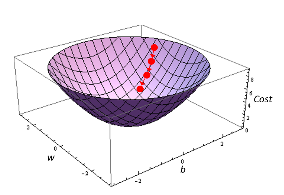
The graph of the cost function now needs another dimension, and so might look like this:

This cost function on a three dimensional graph looks (hopefully) like a bowl, with a minimum point which our computer can try to find using back propagation. As before, we will start at a random point, given by particular values of w and b, as shown by the red dot in the diagram.
Our computer needs to calculate the gradient of the surface of the bowl at this point. Getting the gradient of a surface is easier than it might sound – if you are interested you can look up the gradient (or grad) operator, https://en.wikipedia.org/wiki/Gradient. On the surface our computer needs to find another point close to, and directly ‘downhill’, of our starting point and then calculate the gradient and direction between these points.
With gradient descent our computer can then step down this gradient on the surface of the bowl, to move (hopefully) towards the minimum point in the surface:
This will allow us to find the values of both w and b which correspond to the minimum point on the surface, and then give us the best fit of our prediction to the data.
If we label these best values of w and b as w* and b*, then our equation for predicted pressure y will be:

So our computer has now learned to make predictions of pressure when we have two variables: w and b!
When the cost function depends on one or two variables (just w, or w together with b) at least we can visualise the problem by plotting and 2D or 3D graph of the cost function. Machine learning usually has many, many more variables, so we won’t be able to draw a graph and we will be working blind! We won’t be able to visualise the problem, so we will have to trust that the mathematics that we’ve worked out here can be applied to more complicated problems.
What’s next?
Now that we’ve studied the ideas of the cost function and gradient descent, we can now think again about the cat recogniser challenge that we introduced above. We will understand some basic ideas about neural networks, before we develop these ideas further in a later blog.
Our cat images were 64 x 64 pixels in size, and each pixel had three values for red, green and blue (RGB). This gives a total of 12288 inputs to our neural network.
Rather than draw a neural network with 12288 inputs (which would take an extremely long time to draw!) let’s simply draw just three inputs. We can represent our neural network in a diagram like this:

This neural network has three layers: the input layer, a hidden layer in the middle, and an output layer. Neural networks can be created with any number of layers, and in the last few years more and more layers have been used to create better machine learning: this is called deep learning: Microsoft recently used a neural network with 125 layers!
The input layer has three nodes (labelled Z1,1, Z1,2 and Z1,3) although this is a simplification of the 12288 nodes we need for our cat recogniser challenge. The hidden layer has two nodes, and the output layer has one node. The output layer node can take the values 1 (our computer predicts that the image shows a cat) or 0 (the image is not predicted to show a cat).
The nodes are connected with lines called weights, and the values of these weights are shown with W (between the input layer and hidden layer) and X (between the hidden layer and the output layer). The neural network is called a fully connected network because all nodes are connected by weights to all nodes in the next layer.
The computer can calculate forwards through the neural network. For example, the value at node Z2,1 could be calculated by adding the products of the nodes and weights that feed into it:

(The actual calculations in machine learning to move forwards through a neural network are more complicated, involving bias terms and another function called an activation function. These will be introduced in a later blog when we develop our cat recogniser neural network.)
Once the values of all of the hidden layer nodes have been calculated, the value of the output layer node can be calculated using the same approach.
Our computer can then repeat these calculations for lots of different values of the weights, W and X. This will give us a cost function in terms of the full set of weights, and our computer can then learn using gradient descent to find the minimum point in the cost function. This then gives us the set of weights which make our neural network as accurate as possible in predicting whether an image shows a cat.
With a neural network with 64 x 64 x 3 = 12288 nodes in the input layer, around 20 nodes in the hidden layer, and then one output node, accuracy of around 80% can be achieved in recognising cat images.
So our computer has learned to recognise images of cats!
Of course, there are still many more things that artificial intelligences need to learn. The image below shows Harvey, a black Labrador cross border-collie dog.

The cat recogniser always classifies Harvey as a cat! Harvey is not at all happy about that!
Want to learn more?
If you would like to learn more about artificial intelligence and machine learning, check out these great courses on Coursera:
This is an introductory course in machine learning. It is quite mathematical, but the ideas are accessible to school students who are willing to undertake a small amount of independent study of some of the concepts.
This is a set of five courses which will give you a detailed understanding of neural networks, and provide you with an opportunity to build your own neural network. You’ll also learn to write computer code in Python while working on the courses.
Check out this incredible project, teaching artificial intelligences to play hide and seek! This is a different type of machine learning, called reinforcement learning, often used, for example, to create artificially intelligent enemies in video games.


Comments